
PromQL (Prometheus Query Language) is the query language of Prometheus: it selects time series by their name and their labels, then transforms them to answer an operations question. This lesson takes it from the basics to advanced queries, with examples you can run right away in the interface installed by the lesson Prometheus: metrics and PromQL (in French).
What you will learn
By the end of this lesson, you will be able to write and fix the queries that a dashboard or an alerting rule needs:
- Filter series with label selectors and recognize the four PromQL data types.
- Compute rates, totals and percentiles with
rate(),sum()andhistogram_quantile(). - Pick the right function for the metric type,
rate()for a counter,deriv()for a gauge. - Combine two metrics with operators and vector matching (
on(),ignoring(),group_left). - Write the classic monitoring queries: CPU, memory, error rate, latency and disk space prediction.
- Avoid the traps that produce wrong curves without any error message: division by zero, excessive cardinality and queries that are too costly.
How do you get started with PromQL?
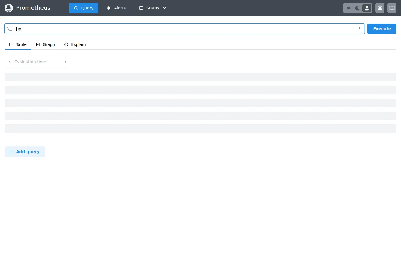
Open the Prometheus interface (http://localhost:9090, or the lab's NodePort
URL) and use the Graph tab to test your queries: the Table view shows
the latest value of each series, the Graph view shows how it evolves.
What is the simplest query?
A metric name on its own is already a complete query: it returns all the series that carry this name, one per combination of labels.
upResult: all the series of the up metric, one per target polled by Prometheus.
up{instance="localhost:9090", job="prometheus"} 1up{instance="node1:9100", job="node"} 1up{instance="node2:9100", job="node"} 0How do you filter with labels?
Label selectors filter the series inside the curly braces. Without a selector, you get every series carrying that metric name, which quickly becomes unreadable on a cluster of several dozen targets.
up{job="node"}Four matching operators exist, two of them based on regular expressions. PromQL regexes are automatically anchored: job=~"node" only matches the exact value node, not node-exporter. This is a classic trap for beginners.
| Operator | Description | Example |
|---|---|---|
= | Exact equality | job="prometheus" |
!= | Not equal to | job!="test" |
=~ | Regex match | job=~"node.*" |
!~ | Regex not match | job!~"test.*" |
Practical examples:
# All HTTP requests except the 200shttp_requests_total{status!="200"}
# GET or POST methodshttp_requests_total{method=~"GET|POST"}
# Namespaces starting with "prod"container_memory_usage_bytes{namespace=~"prod.*"}
What are the PromQL data types?
PromQL handles four data types, and many error messages in the interface come from mixing them up. The first two account for most everyday use: the instant vector represents the current state, the range vector the recent history. Each function expects a precise type as input and produces another as output, which determines which expressions can be nested.
| Type | Description | Example |
|---|---|---|
| Instant vector | Current values (one point per series) | up |
| Range vector | Values over a period | up[5m] |
| Scalar | Floating-point number | 3.14 |
| String | String (rarely used) | "hello" |
Instant vector
This is the most common type: each series carries a single value, the last one known at the evaluation instant.
node_memory_MemAvailable_bytesRange vector
A range vector selects all the values of a series over a period, given
in square brackets. It is the input that functions such as rate() expect.
http_requests_total[5m]The available duration units are s (seconds), m (minutes), h
(hours), d (days), w (weeks) and y (years), and they can be combined:
[1h30m] is a valid window, more readable than a total in minutes.
Which operators does PromQL provide?
Operators let you compute, compare and combine series with each other. Two points set them apart from a classic programming language: they work on sets of series rather than on isolated numbers, and an operation between two metrics only takes place if their labels match. This matching rule explains most of the empty results you get when combining two metrics.
Arithmetic operators
The classic operators apply to each series individually. When one of the two operands is a scalar, the calculation applies to all the series and the metric name disappears from the result, since the value no longer represents the original metric.
# Memory used as a percentage(node_memory_MemTotal_bytes - node_memory_MemAvailable_bytes)  / node_memory_MemTotal_bytes * 100
# Conversion bytes → gigabytesnode_filesystem_size_bytes / 1024 / 1024 / 1024| Operator | Description |
|---|---|
+ | Addition |
- | Subtraction |
* | Multiplication |
/ | Division |
% | Modulo |
^ | Power |
Comparison operators
By default, a comparison filters: it keeps the series that satisfy the condition and drops the others, keeping their original value. This behavior is what makes alerting rules readable, since an alert fires as soon as the result is not empty. The bool modifier changes this: it keeps every series and replaces their value with 0 or 1.
# Instances with CPU > 80%instance:cpu_usage:percent > 80
# Keep only the series above the thresholdhttp_request_duration_seconds > 0.5| Operator | Description |
|---|---|
== | Equal |
!= | Not equal |
> | Greater than |
< | Less than |
>= | Greater than or equal |
<= | Less than or equal |
Logical operators
and, or and unless reason on the presence of series, not on their values, and only apply between two instant vectors. Two series match when all their labels are identical; unless is typically used to exclude from an alert the targets already under maintenance.
# Series present in both (intersection)metric_a and metric_b
# Series present in one or the other (union)metric_a or metric_b
# Series of A absent from Bmetric_a unless metric_b
Which functions do you need first?
A handful of functions is enough for most dashboards and alerts. They fall into two families: those that turn a range vector into an instant vector, such as rate(), and the aggregators that reduce several series to one, such as sum(). The rule to remember is that any counter must go through the first family before it is displayed.
rate(), rate of change
rate() is the function you will use the most: it computes the average per-second
rate of a counter over the given window, compensating for the resets to zero
when the process restarts.
# Requests per second (over 5 minutes)rate(http_requests_total[5m])irate(), instantaneous rate
irate() computes the rate like rate(), but from only the last two
points of the window. It reacts faster to a spike, at the cost of a much
noisier curve: keep it for exploration, not for alerts.
# Instantaneous rate (last 5 min of data)irate(http_requests_total[5m])increase(), total increase
increase() gives the total increase of a counter over the period,
that is the rate from rate() multiplied by the window duration: the
result reads as a number of events, not as events per second.
# Number of requests over 1 hourincrease(http_requests_total[1h])sum(), avg(), min(), max(), aggregations
These aggregators reduce several series to a single value per instant. Without a by or without clause, all labels disappear from the result: you get a single number for the whole fleet, which is rarely what you want on a monitoring graph.
# Total requests (all instances)sum(rate(http_requests_total[5m]))
# Average available memory, all nodes combined (a single value)avg(node_memory_MemAvailable_bytes)
# Same calculation, one value per nodeavg by(instance) (node_memory_MemAvailable_bytes)
# Maximum CPUmax(instance:cpu_usage:percent)
Aggregating by label
The by and without clauses choose the labels kept after
aggregation: by lists the ones you keep, without the ones you drop.
without is more robust when new labels appear, since they
stay in the result.
# Sum per jobsum by(job) (rate(http_requests_total[5m]))
# Sum ignoring the instance labelsum without(instance) (rate(http_requests_total[5m]))
histogram_quantile(), percentiles
histogram_quantile() computes a percentile from the buckets
of a histogram: you pass it the target quantile (0.95 for the P95) and the rate of the
buckets, aggregated while keeping the le label.
# P95 latency per jobhistogram_quantile(0.95,  sum by(job, le) (rate(http_request_duration_seconds_bucket[5m])))
# Global P99histogram_quantile(0.99, sum by(le) (rate(http_request_duration_seconds_bucket[5m])))Math functions
These functions apply point by point to an instant vector and leave the labels intact. They are mostly used to make a graph readable: rounding a value before display, bringing a very wide scale down to a logarithm, or removing the sign of a variation.
| Function | Description | Example |
|---|---|---|
abs() | Absolute value | abs(delta(temp[1h])) |
ceil() | Round up | ceil(value) |
floor() | Round down | floor(value) |
round() | Round | round(value, 0.1) |
ln() | Natural logarithm | ln(value) |
log2() | Base-2 log | log2(value) |
log10() | Base-10 log | log10(value) |
sqrt() | Square root | sqrt(value) |
Time functions
They give access to the Prometheus server clock, expressed in UTC: hour() therefore returns the UTC hour, not the local time of your teams. This is the detail that shifts alerts tied to office hours by one or two hours.
| Function | Description |
|---|---|
time() | Current Unix timestamp |
timestamp() | Timestamp of each sample |
day_of_week() | Day of the week (0-6) |
hour() | Hour (0-23) |
Called with no argument, hour() returns a series with no labels at all. But an and
matches series by their labels: with up, it finds no
pair and the result stays empty. The on() modifier, which matches on an empty
set of labels, fixes the problem (the "Vector matching" section details it
below). Measured on Prometheus
3.9.1: the query up == 1 and hour() >= 0 returns 0 series, whereas
up == 1 and on() hour() >= 0 returns one.
# Alert only during business hours (9 am to 6 pm UTC)up == 0 and on() hour() >= 9 and on() hour() <= 18Functions on range vectors
All these functions take a range vector as input, that is a metric followed by a period in square brackets, and return a displayable instant vector. The _over_time variants suit gauges whose oscillations you want to smooth, while resets() and delta() target counters and gauges respectively.
| Function | Description |
|---|---|
avg_over_time() | Average over the period |
min_over_time() | Minimum over the period |
max_over_time() | Maximum over the period |
sum_over_time() | Sum over the period |
count_over_time() | Number of points |
stddev_over_time() | Standard deviation |
changes() | Number of changes |
resets() | Number of resets (counter) |
delta() | Last minus first difference |
deriv() | Derivative (slope) |
predict_linear() | Linear prediction |
# Average CPU over 1 houravg_over_time(instance:cpu_usage:percent[1h])
# Prediction: disk space in 4hpredict_linear(node_filesystem_avail_bytes[6h], 4*3600)
Which advanced queries should you keep at hand?
The queries below are classics to copy into your dashboards. They all rely on the metrics exposed by node_exporter and by the standard HTTP instrumentation, with names that follow Prometheus conventions. Adapt the label names to your environment before alerting on them: handler, status or namespace vary from one instrumentation library to another.
CPU usage
CPU is not exported directly as a percentage: node_exporter publishes a counter of seconds spent in each mode, including the idle mode. So you compute the idle share, then subtract it from 100.
# CPU percentage used per instance100 - (avg by(instance) (rate(node_cpu_seconds_total{mode="idle"}[5m])) * 100)The query reads from the inside out, in five steps:
node_cpu_seconds_total{mode="idle"}: CPU time in idlerate(...[5m]): per-second rate over 5 minavg by(instance): average of the cores per machine* 100: conversion to a percentage100 - ...: usage = 100% - idle
Memory used
Use MemAvailable and not MemFree: the kernel counts as available the memory occupied by the disk cache, which it will hand back on demand. A calculation based on MemFree triggers permanent alerts on perfectly healthy servers.
# Percentage of memory used(1 - node_memory_MemAvailable_bytes / node_memory_MemTotal_bytes) * 100HTTP error rate
This error ratio is the building block of a service level objective (SLO). Both sum() calls are essential: without them, the division would happen series by series and fail, for lack of identical labels on both sides.
# 5xx error rate over the totalsum(rate(http_requests_total{status=~"5.."}[5m])) / sum(rate(http_requests_total[5m])) * 100P95 latency
The P95 gives the duration under which 95% of requests fall. The le label must stay in the by, otherwise the function loses the bucket bounds and can no longer interpolate; handler then lets you spot the endpoint responsible.
# P95 per endpointhistogram_quantile(0.95, sum by(handler, le) (rate(http_request_duration_seconds_bucket[5m])))Disk space prediction
Alerting on a fixed fill threshold often comes too late. By extrapolating the consumption slope observed over the last six hours, you get a time before saturation, far more actionable. The window must stay wide enough to absorb variations: over one hour, the slightest log rotation skews the projection.
You divide the free space, in bytes, by the speed at which it shrinks,
in bytes per second: the result is a number of seconds. deriv()
is negative when the disk fills up, hence the minus sign that makes the
result positive; a negative result signals on the contrary a disk that is
freeing up.
# Prediction: how long until the disk is full (seconds)node_filesystem_avail_bytes / -deriv(node_filesystem_avail_bytes[6h])Top 5 consumers
topk() recomputes its ranking at every point in time, which makes series appear and disappear along the graph. The container!="" filter discards the series aggregated by cgroup that cAdvisor publishes alongside the containers, and which would duplicate entries in the ranking.
# Top 5 pods by memorytopk(5, container_memory_usage_bytes{container!=""})Queries with offset
The offset modifier shifts the evaluation window into the past, which lets you compare current traffic with the previous week's. This comparison is only valid if your retention period covers the requested shift, otherwise the query returns an empty result.
# Difference with 1 week agorate(http_requests_total[5m]) - rate(http_requests_total[5m] offset 1w)What is vector matching?
When you combine two vectors, PromQL does label matching: for each series on the left, it looks for the series on the right that carries exactly the same labels. No match means no result, with no error message, and this is a frequent cause of empty graphs. The modifiers presented here relax this rule when the two metrics do not share the same set of labels.
One-to-one (default)
By default, matching is one-to-one: each series on the left must find on the right exactly one series carrying the same labels.
# Same labels on both sidesmetric_a / metric_bIgnoring / on
on(...) restricts matching to the listed labels, ignoring(...)
removes from the comparison the ones you name. on() with an empty list
matches on no label, which is used to combine a series with a global
value such as hour().
# Match only on the "job" labelmetric_a / on(job) metric_b
# Match while ignoring the "instance" labelmetric_a / ignoring(instance) metric_b
Group modifiers
When a series on one side must serve several series on the other, PromQL refuses the operation until you say which side carries the multiplicity. group_left designates the left operand as the one that holds several series per match, group_right does the opposite. The classic use is to enrich measurements with the labels of an info metric such as kube_pod_info.
# Several series of A share the same series of B (same job)metric_a / on(job) group_left metric_bWhich PromQL best practices matter?
A correct query can still be costly or misleading. The three points below cover topics that come back regularly in production: naming metrics so they can be guessed, avoiding typing errors that produce credible but wrong curves, and containing the cost of queries. Cardinality, that is the number of distinct series, weighs heavily on Prometheus memory.
Naming metrics
The naming convention is not cosmetic: the unit suffix and the type suffix tell the reader how to query the metric without consulting the exporter's documentation. Prometheus expects base units, that is seconds and bytes, never milliseconds or megabytes.
<namespace>_<name>_<unit>_<suffix>Examples:
http_requests_total(counter)http_request_duration_seconds(histogram)node_memory_MemAvailable_bytes(gauge)
Avoiding common traps
These three mistakes produce no error message: they give a graph that displays normally, with wrong values or a server that saturates. The tabs below set the faulty version against its fix.
Avoid, wrong on a gauge: rate().
rate(node_memory_MemAvailable_bytes[5m]) # WRONGDo, correct for a gauge: deriv().
deriv(node_memory_MemAvailable_bytes[5m])Avoid, risk of NaN when the denominator is zero:
rate(errors[5m]) / rate(requests[5m])Do, version protected against division by zero:
rate(errors[5m]) / (rate(requests[5m]) > 0)or
rate(errors[5m]) / rate(requests[5m]) or vector(0)Avoid, explosive cardinality:
sum by(user_id) (http_requests_total) # Millions of seriesDo, reasonable aggregation:
sum by(endpoint, status) (http_requests_total)Performance
The cost of a query depends on the number of series loaded and on the depth of history scanned. A dashboard refreshed every fifteen seconds replays its queries constantly: what is acceptable in manual exploration becomes a problem once displayed on a wall screen. Recording rules move the computation from display time to ingestion time.
- Use recording rules for frequent complex queries
- Limit the period:
[5m]is often enough - Aggregate early:
sum by(job) (rate(...))rather than computations on all the series - Avoid
.*in regexes: prefer exact values
Cheatsheet
This summary gathers the expressions to keep at hand, grouped by intent. Replace metric, counter and histogram_bucket with your own metric names; the rest of the syntax can be copied as is.
# === COUNTERS ===rate(counter[5m])              # Per-second rateincrease(counter[1h])          # Total increaseirate(counter[5m])             # Instantaneous rate
# === AGGREGATIONS ===sum(metric)                    # Totalavg(metric)                    # Averagemax(metric)                    # Maximummin(metric)                    # Minimumcount(metric)                  # Number of seriessum by(label) (metric)         # Group by label
# === PERCENTILES ===histogram_quantile(0.95, sum by(le) (rate(histogram_bucket[5m])))
# === TIME ===avg_over_time(metric[1h])      # Average over 1hmax_over_time(metric[24h])     # Max over 24hpredict_linear(metric[6h], 3600)  # Prediction in 1h
# === COMPARISON ===metric > 80                    # Filtermetric > bool 80               # Returns 0/1topk(5, metric)                # Top 5bottomk(3, metric)             # Bottom 3
# === LABELS ===label_replace(metric, "new", "$1", "old", "(.*)")label_join(metric, "new", ",", "label1", "label2")
Key takeaways
rate()for counters,deriv()for gaugesby()andwithout()control the aggregationhistogram_quantile()for percentiles, keeping thelelabel- A comparison filters series;
boolreturns 0 or 1 - Two vectors only combine if their labels match:
on(),ignoring()andgroup_leftrelax the rule - Protect divisions against zero
- Test in the interface before setting up an alert